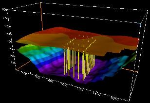
The ice and bedrock surfaces of a portion of the Worthington Glacier obtained in the 1996 radio echo sounding survey. The 1994 boreholes are also plotted. (Plot by Joel Harper, U. of Wyo.) Click on the image for a larger version.
Processing the Radio Echo-Sounding (RES) data transforms the data from incoherent numbers to a data set that can be interpreted. Our processing methods are drawn from refection seismology techniques. These are outlined in Welch, 1996; Welch et al., 1998; and Yilmaz, 1987. We use a number of IDL (from Research Systems, Inc.) scripts to organize our data and usually create screen plots of each profile through each step of the processing to help identify problems or mistakes. We also use Seismic Unix (SU), a collection of freeware seismic processing scripts from the Colorado School of Mines. SU handles the filtering, gain controls, RMS, and migration of the data. IDL is used for file manipulation and plotting and provides a general programming background for the processing.
The processing steps below are listed in the order that they are applied. The steps should be followed in this order. Note that quality of the processing results are strongly dependent on the quality of the field data.
The first step of data processing is to organize and clean the field data so that all the profiles are oriented in the same direction (South to North, for example), any duplicated traces are deleted, profiles that were recorded in multiple files are joined together, and surface coordinates are assigned to each trace based on survey data. These steps are some of the most tedious, but are critical for later migration and interpretation.
The data is plotted as though the transmitter and receiver were a single point and the glacier surface is a horizontal plane. Since neither is the case, the data must be adjucted to reflect actual conditions. The transmitter-receiver separation results in a trigger-delay equivalent to the travel-time of the signal across the distance separating the two. This travel-time is added to the tops of all the traces as a Static Correction.
The data is adjusted with respect to the highest trace elevation in the profile array. Trace elevations are taken from the survey data and the elevation difference between any trace and the highest trace is converted into a travel-time through ice by multiplying the elevation distance by the radio-wave velocity in ice (1.69 x 10⁸ m/s). The travel-time is added to the top of the trace, adjusting the recorded data downward.
We use a bandpass filter in SU to elimitate low and high frequency noise that result from the radar instrumentation, nearby generators, etc. Generally we accept only frequencies within a window of 4-7 MHz as our center transmitter frequency is 5 MHz. Depending on the data, we will adjust the gain on the data, but generally avoid any gain as it also increases noise amplitude. We try to properly adjust gain controls in the field so that later adjustment is unnecessary.
We 2-D migrate the data in the cross-glacier (or across the dominent topography of the dataset) in order to remove geometric errors introduced by the plotting method. Yilmaz (1987) provides a good explanation for the need for migration as well as descriptions of various migration algorithms.
Why is migration necessary?
The radar transmitter emits an omni-directional signal that we can assume is roughly spherical in shape. As the wave propagates outward from the transmitter, the size of the spherical wavefront gets bigger so when it finally reflects off a surface, that surface may be far from directly beneath the transmitter. Since by convention, we plot the data as though all reflections come from directly below the transmitter, we have to adjust the data to show the reflectors in their true positions.
We generally use a TK migration routine that is best for single-velocity media where steep slopes are expected. As you can see from the plot below, the shape of the bed reflector has changed from the unmigrated plots shown in the previous section.
In order to account for the 3-dimensional topography of the glacier bed, we now migrate the profiles again, this time in the down-glacier direction. We use the same migration routine and the cross-glacier migrated profiles as the input. Although not as accurate as a true 3-dimensional migration, this two-pass method accounts for much of the regional topography by migrating in two orthogonal directions. Radar Profile After Down-Glacier Migration
Once the profiles have been migrated in both the cross-glacier and down-glacier directions, we use IDL to plot the profiles as an animation sequence. The animation shows slices of the processed dataset in both the down-glacier and cross-glacier direction. By animating the profiles, it is easier to identify coherent reflection surfaces within the dataset. Another IDL script allows the user to digitize, grid, and plot reflection surfaces.
The resolution of an interpreted surface is a function of the instrumentation, field techniques and processing methods. Through modeling of synthetic radar profiles, we have shown that under ideal circumstances, we can expect to resolve features with a horizontal radius greater than or equal to half the transmitter's wavelength in ice. So for a 5 MHz system, we can expect to resolve features that are larger than about 34 m across. Since the horizontal resolution is far coarser than the vertical resolution of 1/4 wavelength, we use the horizontal resolution as a smoothing window size for the interpreted reflector surfaces. We use a distance-weighted window to smooth the surfaces.
The ice and bedrock surfaces of a portion of the Worthington
Glacier obtained in the 1996 radio echo sounding survey. The 1994
boreholes are also plotted. (Plot by Joel Harper, U. of Wyo.)
Click on the image for a larger version.
![]() Return to Main
Radio-Echo Sounding Page
Return to Main
Radio-Echo Sounding Page
Updated: August 3, 2011
© 1998, Brian C. Welch,
Univ. of Wyoming